
Stock valuation formulas: DDM, DCF and P/E

Key Takeaways
- DDM and FCFE estimate the equity claim using the cost of equity; FCFF uses the weighted average cost of capital before a bridge to equity.
- A constant-growth formula requires a discount rate above its growth rate and a sustainable cash-flow assumption.
- A P/E-based estimate multiplies matching EPS by a selected multiple; the selection still needs justification.
Research Scope
- Regions
- General nonfinancial-company methods; USD used only for hypothetical arithmetic. No live market or issuer dataset.
- Period
- Sources accessed October 15, 2026. Annual end-of-year cash flows and annual rates in every example.
- Industries
- Industrial and resource-company research; application notes are analytical guidance, not accounting advice.
- Data objects
- Dividends, FCFE, FCFF, equity cost, WACC, growth, terminal value, common shares and P/E.
Mixing an equity cash flow with a firm discount rate changes the answer before any forecast is tested. A stock valuation formula must match the claim being valued: use dividends or free cash flow to equity with the cost of equity, or free cash flow to the firm with the weighted average cost of capital before converting to equity.
For a direct per-share estimate, the constant-growth dividend formula is V₀ = D₁ ÷ (kₑ − g). A broader DCF discounts a forecast cash-flow stream plus its terminal value. A P/E estimate is EPS × a selected P/E multiple. Choose among them by the cash flows you can support, then check the rate, time period and units. The valuation research guide places these calculations within the wider disclosure-reading process.
Compare the formulas before entering numbers
The same algebra can price different claims. Label the cash flow and output before using a spreadsheet cell called “value.”
Scroll horizontally to view all columns.
| Method | Formula | Inputs and rate | Output and condition |
|---|---|---|---|
| Constant-growth DDM | V₀ = D₁ ÷ (kₑ − g) | Next annual dividend per share; annual equity cost kₑ; perpetual dividend growth g | Currency per share; kₑ > g and a supportable continuing payout |
| Equity DCF | E₀ = Σ FCFEₜ/(1+kₑ)ᵗ + TVₙ/(1+kₑ)ⁿ | Cash left for equity after reinvestment and financing; equity cost | Total equity if cash flows are totals; per share if consistently per-share inputs |
| Firm DCF | O₀ = Σ FCFFₜ/(1+WACC)ᵗ + TVₙ/(1+WACC)ⁿ | Operating cash flow after tax and reinvestment, before debt payments; WACC | Operating-asset value; reconcile other assets and claims to obtain common equity |
| P/E estimate | Estimated share value = EPS × selected P/E | A defined earnings period and a multiple on the same basis | Currency per share; meaningful positive earnings and a defensible comparison |
Here, Σ adds forecast years 1 through n, t identifies a year, and TVₙ is the value of later cash flows measured at the end of year n. DDM is itself a form of equity DCF. The firm/equity split follows Damodaran’s introduction; the terminal-value structure follows his public valuation lecture, both accessed October 15, 2026.
Keep an input log beside the formula. A reported dividend, a forecast dividend and an assumed growth rate have different evidential status, even when all three occupy adjacent cells. What a company valuation has to identify explains that distinction.
One hypothetical industrial company for every example
All amounts below are invented teaching assumptions for one mature industrial company. They are not disclosures, market prices or suggested valuation parameters. Cash flows arrive at year-end; the share count stays fixed. The company is assumed to sustain the stated growth after reinvestment and financing.
Scroll horizontally to view all columns.
| Input | Hypothetical value | Role |
|---|---|---|
| Common shares | 2.00 million shares | Converts total equity to a per-share amount |
| Next-year dividend D₁ | USD 2.10 per share | First DDM cash flow |
| Next-year FCFE | USD 4.20 million | Available to common equity; entirely distributed in this example |
| Next-year FCFF | USD 7.00 million | Available to capital providers before debt payments |
| Next-year EPS | USD 2.50 per share | Earnings basis for the assumed leading P/E |
| Equity cost kₑ | 10% per year | Discounts equity cash flows |
| WACC | 8% per year | Discounts firm cash flows |
| Continuing growth g | 3% per year | Assumed for dividends, FCFE and FCFF |
| Debt; excess cash; other claims | USD 80 million; zero; zero | Simplifies the operating-value-to-equity bridge |
| Selected leading P/E | 12× | An assumption applied to next-year EPS |
These inputs were deliberately selected to reconcile. Matching answers therefore demonstrate the arithmetic, not independent evidence that any real stock has that value. For a real issuer, the forecasts, capital structure and discount rates must also agree with one another.
DDM: use the next dividend and test the denominator
The constant-growth dividend discount model divides next year’s dividend by equity cost minus perpetual dividend growth. The CFA Institute’s public 2026 refresher gives this equation with kₑ > g and describes its use for a discernible dividend policy related to profitability.
For the hypothetical company:
V₀ = USD 2.10 per share ÷ (0.10 − 0.03) = USD 30.00 per share.
D₁ is the next dividend, not the last payment. If the starting input is the most recent annual dividend D₀, calculate D₁ = D₀ × (1+g) under the same growth assumption. A quarterly payment needs an explicit annual forecast; a quarterly amount cannot silently become the annual numerator.

This model assumes a continuing distribution stream. A company retaining cash for new capacity may need an explicit forecast of when distributions begin, or an FCFE model. Entering a zero current dividend into the constant-growth shortcut does not establish that the business has zero value.
What happens when growth reaches the discount rate?
The shortcut fails when kₑ ≤ g. At g = 10% and kₑ = 10%, its denominator is zero. At g = 11%, the mechanical result is USD 2.10 ÷ −0.01 = −USD 210 per share, but the assumed infinite dividend stream has no finite present value under this model. That negative number is an invalid model output, not an economic estimate.
Even valid inputs can be sensitive. Holding D₁ at USD 2.10 and kₑ at 10%, hypothetical growth assumptions of 2%, 3% and 4% produce USD 26.25, USD 30.00 and USD 35.00 per share. This is a controlled sensitivity calculation; the three growth rates are not forecasts.
DCF: distinguish equity cash flows from firm cash flows
An FCFE model values equity directly; an FCFF model first values operations. Damodaran’s equity-valuation framework pairs FCFE with equity cost and FCFF with WACC. Interest and debt repayment belong in the equity cash-flow calculation, while the firm calculation is before those financing payments.
For a stable FCFE stream, the hypothetical company’s total equity is:
E₀ = USD 4.20 million ÷ (0.10 − 0.03) = USD 60.00 million.
Dividing by 2.00 million shares gives USD 30.00 per share. DDM agrees here because all FCFE is paid as dividends. If payouts differ from cash available to equity, that equivalence needs investigation.
Calculate terminal value at its own date
A continuing-growth FCFF terminal value uses the first cash flow after the explicit forecast: TVₙ = FCFFₙ₊₁ ÷ (WACC − g), with WACC > g. Then discount TVₙ back n periods, alongside the explicit forecast cash flows.
Using the same company’s 3% growth and 8% WACC, split its continuing stream after two years. All amounts in this calculation are USD millions:
Scroll horizontally to view all columns.
| Item | Calculation | Amount |
|---|---|---|
| Year 1 FCFF | Assumed | 7.0000 |
| Year 2 FCFF | 7.0000 × 1.03 | 7.2100 |
| Year 3 FCFF | 7.2100 × 1.03 | 7.4263 |
| Terminal value at end of year 2 | 7.4263 ÷ (0.08 − 0.03) | 148.5260 |
| Present value of operations | 7/1.08 + 7.21/1.08² + 148.526/1.08² | 140.0000 |
| Common equity | 140 − 80 debt + 0 excess cash − 0 other claims | 60.0000 |
The equity result is again USD 30.00 per share. The operating value also equals 7 ÷ (0.08 − 0.03) = USD 140 million because this constructed example has the same growth and discount rate throughout. Splitting it into forecast and terminal periods simply exposes the dates.
Do not add USD 148.526 million directly to today’s forecast present values: it is a year-2 value. Do not count year-3 cash flow separately as well as inside the terminal value. And do not subtract debt again from an FCFE result, which already values the equity claim.
Deduct reinvestment before calling the cash flow free
For an ordinary nonfinancial operating business, a simplified FCFF construction is after-tax operating earnings + depreciation − capital expenditure − increase in noncash operating working capital. It assumes consistent definitions and a reconciled tax treatment. The firm’s forecast needs those investment outflows to support the growth it assumes.

For industrial research, investigate equipment upkeep and working-capital needs before treating earnings as distributable cash. For resource research, also ask whether asset life supports a perpetual terminal assumption. These are analytical checks, not accounting advice. The EBITDA valuation guide explains why an operating earnings subtotal can leave capital spending unresolved.
P/E: separate the observed ratio from the assumed multiple
P/E = share price ÷ EPS describes a price relative to earnings. Rearranging it gives an estimate only after selecting a multiple: estimated share value = EPS × selected P/E. OpenStax’s P/E explanation distinguishes trailing reported earnings from leading forecast earnings.
For the same hypothetical company, next-year EPS of USD 2.50 × an assumed leading P/E of 12 = USD 30.00 per share. Twelve is a teaching assumption, not an industry benchmark. Using an observed price to calculate P/E and multiplying that same P/E by the same EPS merely returns the starting price.
A loss or near-zero EPS can make the comparison unusable or unstable. A peak-cycle EPS also needs investigation before extrapolation. Use the valuation multiples guide for numerator/denominator selection and sample comparability; this page supplies no sector multiple table.
Check the inputs before interpreting the answer
The most useful final check is to trace each result back to a defined input and date. Leave a missing input blank until it can be supported.
Scroll horizontally to view all columns.
| Check | Record before calculating |
|---|---|
| Claim and perimeter | Operating assets, all equity, or common equity; consolidated scope and excluded assets |
| Cash-flow/rate pairing | FCFF with WACC; FCFE or dividends with equity cost |
| Units | Total currency or currency per share; share count in matching units |
| Time and currency | Annual versus quarterly; valuation date; consistent forecast currency and discount-rate basis |
| Earnings basis | Trailing, forward or normalized; adjustments and forecast source |
| Growth and reinvestment | Investment needed to sustain growth; stable-growth start date; discount rate above perpetual growth |
| Equity bridge | Debt, excess cash, preferred claims, minority interests or other adjustments relevant to the chosen perimeter; avoid double counting |
| Uncertainty | Alternative assumptions and the evidence needed to narrow them |
For a cyclical industrial or resource business, record why the earnings year represents the cycle. If a single year’s profit dominates the estimate, return to the input log and test a different earnings assumption. A small spread between the discount rate and perpetual growth calls for more scrutiny, not extra decimal places.
Method and sources
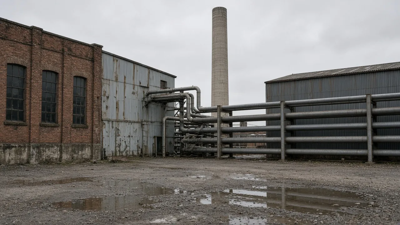
This is a public-source explanation with original hypothetical arithmetic, updated October 15, 2026. The formulas follow the specific Damodaran, CFA Institute and OpenStax pages linked above and listed below, accessed on that date. No current issuer, market rate, commodity forecast or investment return was estimated. The photographs introduce research inputs, distributions and physical reinvestment; they are not source documents or evidence for the numerical example.
For the McKinsey reference, the bibliographic record is: Tim Koller, Marc Goedhart and David Wessels, Valuation: Measuring and Managing the Value of Companies, eighth edition, Wiley, May 2025. This is confirmed by McKinsey’s May 10, 2025 announcement, accessed October 15, 2026. Only that announcement was opened for the citation; no book chapter is summarized here.
To use these methods in research, begin with the input log, select the claim and model, and recalculate under alternative assumptions. The research disclaimer applies throughout: this page provides education, without a buy, sell or hold recommendation.
Continue the research
Related Research

What is the valuation of a company?
What has to be written down before a company valuation figure can be compared with another figure?

Company valuation multiples: pair the claim with the measure
Which valuation multiple matches the claim, and what has to be written down before an industry figure is copied?
EBITDA valuation: same EBITDA, different maintenance cash
How does an EV/EBITDA multiple price an industrial or resource firm, and what does the same EBITDA hide when maintenance cash differs?
Sources & Data Notes
-
Claim and discount-rate pairing; reinvestment and growth consistency.
-
Public course material; no current market parameter is adopted.
-
Only the public introduction and summary were used, not the full paid curriculum.
-
Bibliographic confirmation only: authors, title, eighth edition, Wiley, May 2025. Full book not read.